In this post, I want to kind of bring together the theme of curvature and the theme of affine or projective geometry. My goal is to introduce the spaces of constant curvature as subspaces of Euclidean space and explore their symmetries as groups of matrices.
Table of Contents
1. The $n$-sphere in \(\mathbb{R}^{n+1}\)
Remember our equation for the unit circle? \(x^2 + y^2 = 1\)? This curve is a $1$-dimensional object living in \(\mathbb{R}^2\), affectionately known as \(\mathbb{R}^{1+1}\) and we can easily generalize this equation to \(\mathbb{R}^{n+1}\) as \(x_1^2 + \cdots + x_{n+1}^2 = 1\). This is the $n$-sphere sitting inside \(\mathbb{R}^{n+1}\). For, like, precisely two values of \(n\), we know what to expect: the unit circle in \(\mathbb{R}^2\) and the unit sphere in \(\mathbb{R}^3\). It’s a joy to imagine what the unit $n$-sphere feels like for other values of \(n\). For example, there ought to be a $0$-sphere in \(\mathbb{R}^{0+1}\), and indeed there is: the two points \(x\) such that \(x^2 = 1\). Or the $3$-sphere, which is somehow like and unlike $3$-dimensional space.
If you’ll permit me an aside, here is my favorite way to think of the $3$-sphere; actually it works for \(n\) arbitrary, but for \(3\) I can really picture something if I wrack my brain a little. Let’s go back to the circle: pick a point on the circle, like say the point \((0,1)\), and throw it away. What you’re left with, if you kind of sit with it for a moment, is kind of like an open interval in \(\mathbb{R}\), just curled up funny. Actually, you can do something pretty neat with these leftover points, called stereographic projection. Imagine you’re a little surveyor standing at the point \((0,1)\) in \(\mathbb{R}^2\), and for each other point \((p,q)\) on the circle, it’s your job to first draw the straight line from \((0,1)\) to \((p,q)\), and then second, note down where that line hits the $x$-axis.
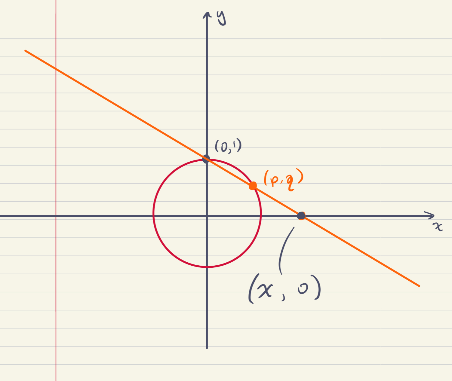
An equation for an arbitrary point on this line is \((tp, tq + (1 - t))\), so the point \((x,0)\) on the line will be such that \(x = tp\) and \(tq + (1 - t) = 0\). This latter equation implies that \(t = \frac{1}{1 - q}\), so \(x = \frac{p}{1 - q}\).
In \(n\) dimensions, the equation for the line becomes \((tx_1,\ldots,tx_n,tx_{n+1} + (1 - t))\), and the point on the hyperplane \(x_{n+1} = 0\) is \((\frac{x_1}{1 - x_{n+1}},\ldots,\frac{x_n}{1 - x_{n+1}},0)\).
Anyway, it's clear that you can reverse this process: for any point \(\vec p\) on the hyperplane \(x_{n+1} = 0\), there is a unique point \(\vec q\) on the unit $n$-sphere such that stereographic projection from \((\vec 0, 1)\) through \(\vec q\) yields \(\vec p\). As the point \(\vec q\) gets closer and closer to \((0,1)\), the point \(\vec p\) goes “off to infinity”. Thus, one way to think of the $n$-sphere is like $n$-dimensional space with one extra point at infinity that “wraps it all up”. Like, the circle is the real line \(\mathbb{R}\) wrapped up with one extra point, the sphere is the plane wrapped up with one extra point… and \(S^3\), the $3$-sphere, is \(\mathbb{R}^3\) wrapped up with one extra point. Neat, huh?
Anyway, consider a linear transformation of \(\mathbb{R}^{n+1}\). There are many such, and all of them may be represented by \((n+1)\times(n+1)\) matrices! The action of the transformation on \(\mathbb{R}^{n+1}\) is matrix multiplication. I mean, the point of this post is we all love linear algebra, right? Anyway, suppose we want two things to happen: first, our transformation (or equivalently our matrix \(M\)) should be invertible in the sense that we can undo it. In terms of the matrix, this means that there exists a matrix \(M^{-1}\) such that \(MM^{-1} = M^{-1}M = I\), the identity matrix. If you remember linear algebra, you might know that this comes down to a condition on the determinant of \(M\): that determinant must not be \(0\).
The other thing we want to have happen is that the matrix preserves the unit sphere. But the equation \(x_1^2 + \cdots + x_{n+1}^2 = 1\) has a vector interpretation: if \(\vec x = (x_1,\ldots,x_n)\), we have that the coordinates of \(\vec x\) satisfy the equation for the unit sphere if and only if the dot product \(\vec x \cdot \vec x = x_1^2 + \cdots + x_{n+1}^2\) is \(1\). This dot product may also be expressed as a matrix product \(\vec x^T \vec x = 1\), where we think of \(\vec x\) as a column vector and \(\vec x^T\), its transpose, as the corresponding row vector. Sneakily, we can put in any \((n+1)\times(n+1)\) matrix between \(\vec x^T\) and \(\vec x\) and we’ll end up with a number. To make sure we end up with the same number, let’s just put \(I\), the identity matrix \(\begin{pmatrix} 1 & 0 & \cdots & 0 \\ 0 & 1 & \cdots & 0 \\ \vdots & \vdots & \ddots & \vdots \\ 0 & 0 & \cdots & 1 \end{pmatrix}\) there.
Anyway, we want \(M\vec x \cdot M \vec x = {(M \vec x)}^T M\vec x = \vec x^T M^TIM \vec x = \vec x^T \vec x = 1\). This turns out to happen just when \(M^TM = I\). Actually this implies that \(M\) is invertible, and furthermore that \(MM^T = I\) as well, so that \(M^T\) is actually the inverse of \(M\).
Let’s suppose we’re working with the unit circle in \(\mathbb{R}^2\) and that we have a symmetry \(M\) which sends the point \((1,0)\) to \((p,q)\). Recall that this actually means that the first column of \(M\) is \((p,q)\)! Since we need \(M^TM = I\), if the other column of \(M\) is \((c,d)\), we compute
\(M^TM = \begin{pmatrix}p & q \\c & d\end{pmatrix}\cdot\begin{pmatrix}p & c \\q & d\end{pmatrix} = \begin{pmatrix} p^2 + q^2 & pc + qd \\ cp + dq & c^2 + d^2 \end{pmatrix} = \begin{pmatrix} 1 & 0 \\ 0 & 1 \end{pmatrix}\)
Since \(p^2 + q^2 = 1\), one of \(p\) or \(q\) is nonzero, so we can divide by it to see that (supposing it is \(p\)) \(c = -\frac{qd}{p}\). Then \(c^2 + d^2 = 1\) implies \(\frac{q^2d^2}{p^2} + d^2 = 1\), so (doing some tricksy algebra) \(d^2 = p^2\). So either \(d = p\), in which case \(c = -q\), or \(d = -p\), in which case \(d = q\). That is, there are exactly two choices for \(M\), \(\begin{pmatrix}p & -q \\ q & p\end{pmatrix}\) and \(\begin{pmatrix}p & q \\ q & -p\end{pmatrix}\). These are distinguished by the sign of their determinant or equivalently by whether they “preserve or reverse orientation”, meaning that one of them is more like a rotation, while the other is a rotation followed by a flip.
Notice as well that if a matrix \(M\) preserves the $n$-sphere in \(\mathbb{R}^{n+1}\), it actually preserves the set of points satisfying \(x_1^2 + \cdots + x_{n+1}^2 = r^2\) for all \(r\)!
We can think of the $n$-sphere, \(S^n\) as a metric space in two ways. The first is to restrict the metric from Euclidean space to the sphere. This works fine, but is a little weird: the distance then on the circle from \((0,1)\) to \((1,0)\), say, is \(\sqrt{2}\), but the actual shortest path on the circle from \((0,1)\) to \((1,0)\) is longer; in fact it has length equal to the arc length of the curve tracing out the part of the circle from \((0,1)\) to \((1,0)\). Since we “know” that the perimeter of a circle is \(2\pi\) times its radius and this curve is a quarter of that circle, we should expect the distance between \((0,1)\) and \((1,0)\) to be \(\frac{pi}{2}\).
This latter distance, measuring the angle between \(\vec p\) and \(\vec q\), is connected to their dot product. For the unit sphere in \(\mathbb{R}^{n+1}\), we have that this angle \(\theta\) satisfies \(\vec p \cdot \vec q = \cos\theta\). (In general one has to account for the norms of \(\vec p\) and \(\vec q\).) Anyway, this distance \(d(\vec p, \vec q) = \arccos(\vec p \cdot \vec q)\), is called the round metric on the unit $n$-sphere in \(\mathbb{R}^{n+1}\). With respect to this metric, the embedding of \(S^n\) into \(\mathbb{R}^{n+1}\) is an isometric embedding, and by our earlier calculations of curvature, we see that \(S^n\) equipped with this metric has constant sectional curvature \(1\).
2. Euclidean space
As we've seen in previous posts, there is a useful way of thinking of affine subspaces of \(\mathbb{R}^n\) as linear subspaces of \(\mathbb{R}^{n+1}\), namely if \(p_1,\ldots,p_k\) are affinely independent points in \(\mathbb{R}^n\), the subspace that they generate may be thought of as the linear subspace of \(\mathbb{R}^{n+1}\) spanned by the vectors \(v_1,\ldots,v_k\), where \(v_i = (p_i, 1)\). That is, \(v_i\) is the vector whose first \(n\) coordinates are the coordinates of the point \(p_i\) and whose last coordinate is \(1\). One reason for setting the last coordinate to something nonzero is that if one of the \(p_i\) is the origin, thinking of it as a vector is unproductive: the zero vector is never part of a linearly independent set.
Thus the line in \(\mathbb{R}^2\) through the points \((3,7)\) and \((4,5)\) corresponds to the linear subspace (a plane) in \(\mathbb{R}^3\) spanned by the vectors \((3,7,1)\) and \((4,5,1)\). (Strictly speaking, we should be careful to think of vectors as either row or column vectors, but I am assuming here that you don't care either.) Indeed, if you look at this plane in \(\mathbb{R}^3\), the places where it slices through the plane \(z = 1\) in \(\mathbb{R}^3\) forms a line which passes through the given points.
Consider the (column) vector \(\vec v = (x, y, z)\) and a \(3\times3\) matrix \(M\). The last coordinate of the matrix \(M\vec v\) is the dot product of the last row of \(M\) (thought of as a column vector) with \(\vec v\). In other words, if the last row of \(M\) is \((m_{31}, m_{32}, m_{33})\), we have that the last coordinate of \(M\vec v\) is \(m_{31}x + m_{32}y + m_{33}z\).
Suppose that the first two entries, \(x\) and \(y\) of \(\vec v\) are allowed to be arbitrary—whatever numbers you want—but that \(z = 1\). For \(M\) to preserve this property, that is, for \(M\) to send the \(z = 1\) plane in \(\mathbb{R}^3\) to itself, we see that we must have \(m_{31} = m_{32} = 0\), while \(m_{33} = 1\). In other words, we can write \(M\) in block form as \(\begin{pmatrix} A & \vec w \\ \vec 0 & 1 \end{pmatrix}\), where \(A\) is a \(2\times2\) matrix, \(\vec w\) is a \(2\times 1\) matrix (affectionately known as a column vector), \(\vec 0\) is the zero \(1 \times 2\) row vector and \(1\) is, well, \(1\). Invertible matrices of this form are part of the affine group, which is so named because it preserves the affine plane \(z = 1\). In fact, for a matrix of this form to be invertible, it turns out to suffice to ask that \(A\) is invertible. Indeed, doing block matrix multiplication we see that
\(\begin{pmatrix} A^{-1} & -A^{-1}\vec w \\ \vec 0 & 1\end{pmatrix}\begin{pmatrix} A & \vec w \\ \vec 0 & 1\end{pmatrix} =\begin{pmatrix} A^{-1}A & A^{-1}\vec w - A^{-1}\vec w \\ 0 & 1\end{pmatrix} = I\).
Anyway, to be a rigid motion of Euclidean space, we want distances to be preserved. Recall that the distance between vectors \(\vec v\) and \(\vec w\) is \(\|\vec v - \vec w\| = \sqrt{(\vec v - \vec w) \cdot (\vec v - \vec w)}\). Notice that for vectors on the affine plane \(z = 0\), the distance between vectors corresponds to the usual Euclidean distance between points on the plane. In other words \(d((\vec v, 1), (\vec w, 1)) = d(\vec v, \vec w)\), because the last coordinate becomes zero.
Doing a little matrix multiplication, we see that in \(n\) dimensions, the image of the vector \((\vec v, 1)\) under the matrix \(M\) above is \((A\vec v + \vec w, 1)\). Therefore the matrix \(M\) will preserve distances on the hyperplane \(x_{n+1} = 1\) just when the matrix \(A\) satisfies \(A\vec v \cdot A \vec v = \vec v \cdot \vec v\). In other words, the matrix \(A\) actually be one that preserves the $(n-1)$-sphere in \(\mathbb{R}^n\)! That’s pretty neat.
Actually, before I go on to talk about hyperbolic space, I want to point out a neat fact: Since \(AA^T = 1\), doing block-matrix multiplication, we see that
\(M\begin{pmatrix}I & 0 \\ 0 & 0 \end{pmatrix}M^T = \begin{pmatrix}A & \vec w \\ \vec 0 & 1\end{pmatrix}\begin{pmatrix}A^T & \vec 0\\ \vec 0 & 0 \end{pmatrix} = \begin{pmatrix} I & \vec 0 \\ \vec 0 & 0 \end{pmatrix}\).
Actually, writing \(g\) for the matrix \(\begin{pmatrix}I & \vec 0 \\ \vec 0 & 0 \end{pmatrix}\), we see that a matrix \(M\) preserving the hyperplane \(x_{n+1} = 1\) is a rigid motion of Euclidean space if and only if it satisfies \(MgM^T = g\).
3. Hyperbolic space
Okay, bear with me, this one is kind of weird but also very very cool. Earlier, when we stipulated that an \((n+1)\times(n+1)\) matrix \(M\) belonged to the symmetry group of \(S^n\) when it satisfied \(M^T I M = I\) or \(M I M^T = I\), we actually may replace \(I\) with any \((n+1)\times(n+1)\) matrix we’d like. We already did this a little right at the end of the previous section, where \(I\) was replaced with \(g\), the matrix whose first \(n\) diagonal entries are \(1\) and whose last entry is \(0\). Interestingly, when that last entry is \(1\), we had a space with “constant sectional curvature equal to \(1\)”, when we gave it the round metric. and when it was \(0\), we got a space with constant sectional curvature equal to \(0\). It’s extremely tempting to see what might happen if we let that last entry be \(-1\) instead!
So let \(g\) be the matrix \(\begin{pmatrix}I & \vec 0 \\ \vec 0 & -1 \end{pmatrix}\) and suppose \(M\) is a matrix satisfying \(M^TgM = g\). Notice that \(M\) preserves the (one-sheeted) hyperboloid comprising those points in \(\mathbb{R}^{n+1}\) satisfying \(x_1^2 + \cdots + x_n^2 - x_{n+1}^2 = 1\): these are just the vectors \(\vec x\) for which \(\vec x^T g \vec x = 1\). But actually it also preserves the two-sheeted hyperboloid \(x_{n+1}^2 - x_1^2 - \cdots - x_n^2 = 1\). One way to see this is to note that it is the set of vectors for which \(\vec x^T g \vec x = -1\), and if \(M^TgM = g\), then \(\vec x^T g \vec x = \vec x^T M^TgM \vec x\), so if the left hand equation is \(-1\), so is the right-hand equation.
One reason to prefer the two-sheeted hyperboloid is that it doesn’t have a “hole”, and another is that, like the sphere \(S^n\) and \(\mathbb{R}^n\) as the hyperplane \(x_{n+1} = 1\), the two-sheeted hyperboloid includes the point \((\vec 0, 1)\).
Since \(g\) is invertible, the equation \(M^T g M = g\) implies that \(M\) is invertible. The group of matrices satisfying \(M^TgM = g\) is kind of curious: an element of this group may swap the two sheets of the hyperboloid, or it may fix them. Let’s suppose it fixes them, so that \(\vec v_{n+1} > 0\) implies that \({(M\vec v)}_{n+1} > 0\).
3.1. A metric on hyperbolic space
Just as we found the round metric on the $n$-sphere in \(\mathbb{R}^{n+1}\), it would be nice to have a formula for the distance between two points on the hyperboloid. It’s a little tough to know precisely what we’re asking for here, but one reasonable thing to ask would be for linear subspaces of \(\mathbb{R}^{n+1}\), when intersected with one of the sheets of the hyperboloid, to be convex in the hyperboloid, in the sense that the “shortest path” in this metric should stay within this linear subspace. In particular, if we set one of our points to be \((\vec 0, 1)\), the other point will lie on a sub-hyperbola of the hyperboloid.
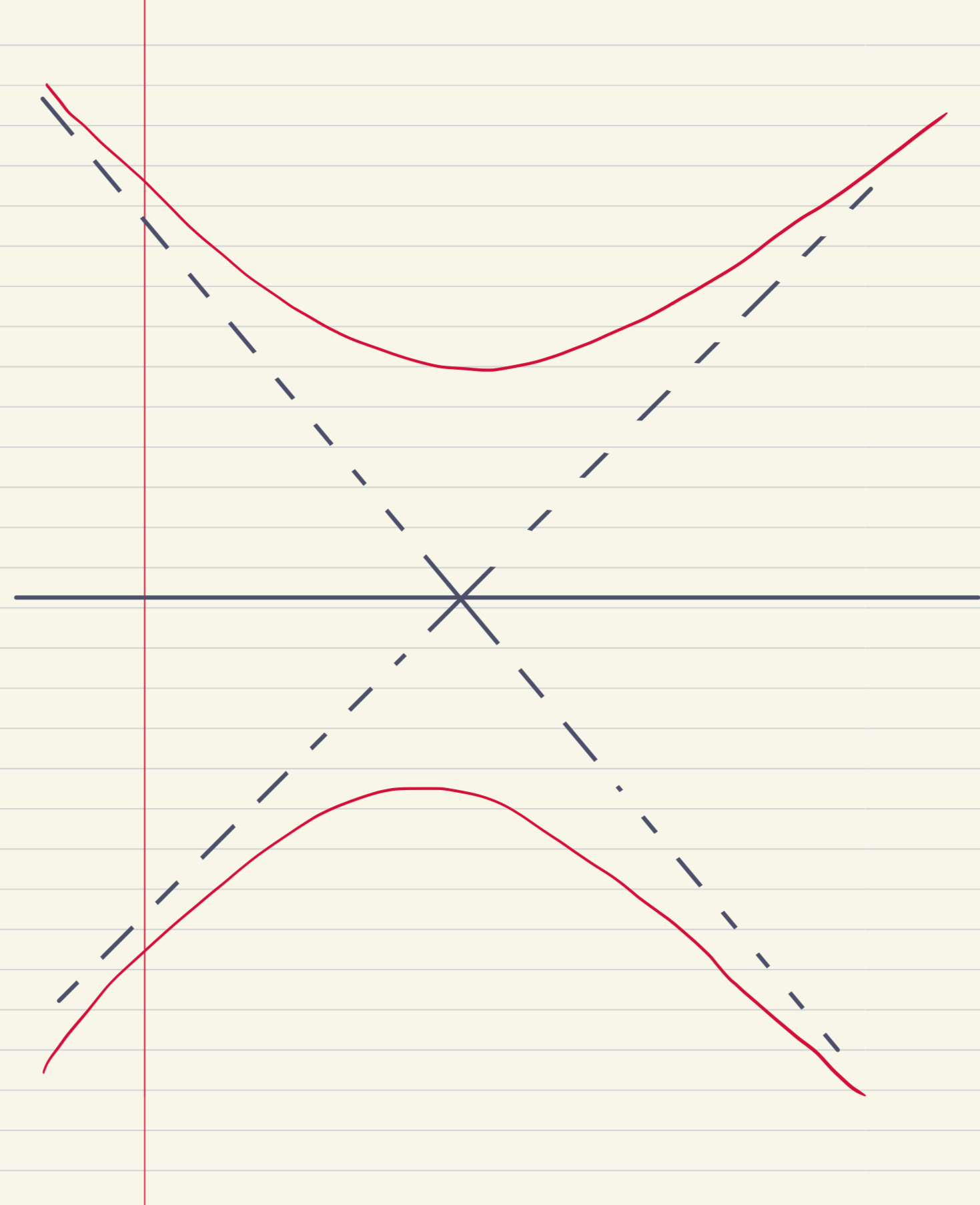
That is, let’s think in \(\mathbb{R}^2\). There are many ways to parametrize the hyperbola, but I’d like to argue that the best one is maybe the weirdest: \(t \mapsto (\sinh t, \cosh t)\). The functions \(\cosh\) and \(\sinh\) are pronounced “cosh” (like as in “oshkosh”) and “cinch” (like as in “it’ll be a cinch!” maybe more phonetically “sin-tch”). You maybe met them in a Calculus class once upon a time and they’re defined as
\(\cosh x = \frac{e^{x} + e^{-x}}{2}\) and \(\sinh x = \frac{e^{x} - e^{-x}}{2}\).
Let’s do a little math, shall we? First of all notice that \(e^{-x} = \frac{1}{e^x}\), so if we write \(a = e^x\), we can compute
\[\sinh^2 x - \cosh^2 x = \frac{{(a - \frac{1}{a})}^2}{4} - \frac{{(a + \frac{1}{a})}^2}{4} = \frac{a^2 - 2 + \frac{1}{a^2}}{4} - \frac{a^2 + 2 + \frac{1}{a^2}}{4} = -\frac{4}{4} = -1\].
Therefore this really is the parametrization of the upper sheet of the hyperboloid.
The reason I prefer this parametrization is that the derivative of \(\sinh t\) with respect to \(t\) is, one checks, \(\cosh t\) and vice versa. Thus the velocity vector of the curve \(t \mapsto (\sinh t, \cosh t)\) is \(\vec v = (\cosh t, \sinh t)\), which satisfies \(\vec v^T g \vec v = 1\). In other words, with respect to a funky way \(g\) of measuring “norms” of vectors, the vector \(\vec v\) is a unit vector.
This is significant, because it says that with respect to our funky norm, the curve \(t \mapsto (\sinh t, \cosh t)\) is parametrized by arc length. In other words, we can define a distance between points \((\sinh s, \cosh s)\) and \((\sinh t, \cosh t)\) on the hyperbola as \(|s - t|\)!
If we let \(s = 0\), notice that this quantity, \(|t|\), is related to the $y$-coordinate of the point \((p,q) = (\sinh t, \cosh t)\) whose distance to \((0,1)\) we are trying to measure. In fact, we have
\[\sinh s \sinh t - \cosh s \cosh t = -\frac{e^{s - t} + e^{t - s}}{2} = -\cosh (s - t),\]
so we can compute this distance based on knowing the vectors \(\vec v\) and \(\vec w\) as \(\operatorname{arccosh} (-\vec v^T g \vec w)\).
As it turns out, this metric on the hyperboloid turns it into a Riemannian manifold of dimension \(n\) and constant sectional curvature \(-1\). Since, as it turns out, the embedding of the hyperboloid into \(\mathbb{R}^{n+1}\) is not isometric, we can't compute this directly from the definition of the hyperboloid. This is maybe one situation where the curvature tensor actually turns out to be useful.
There's much more I'd like to say about hyperbolic space, but this post is long in the tooth as it is, so I'll sign off here for now.