As a geometric group theorist interested in “CAT(0)” and “hyperbolic geometry”, I appear to care very deeply about notions like “curvature”, but I have to admit my understanding of what it means is not that deep. This post is an attempt (one of likely several) to deepen my understanding. I’d like to bring you along for the ride.
Table of Contents
1. Curves
1.1. Curvature of curves is not intrinsic
In differential geometry classes, curvature is often mooted as an inherently two-dimensional phenomenon, or rather, one that begins at dimension two. Yet, the word that mathematicians use to describe one-dimensional shapes sitting inside another shape is curve. This is maybe a silly way of arguing, but I think this use of language suggests that curvature should have a one-dimensional meaning. Indeed, the point of a “curve” is that it is not “straight” (although perversely, for a mathematician a straight line counts as a curve).
So what gives? The reason for this is that in dimension one, curvature is an “extrinsic” phenomenon.
Let me explain. First, let’s make sense of what it would mean for something to be an intrinsic property. Consider the real line. Mathematicians usually denote it \(\mathbb{R}\) for “real”, sometimes decorated as \(\mathbb{R}^1\) to indicate the dimension and distinguish it from something like the Cartesian plane \(\mathbb{R}^2\) and so on. For a mathematician, \(\mathbb{R}\) lives “off by itself”. Although we as humans typically reason about things spatially, it’s important to be able to discard what is not part of the definition of \(\mathbb{R}\) and retain only what is. In other words, when I said “consider the real line”, maybe you imagined a line living inside a three-dimensional space (I like to think pictorially, so I know I did this). But the point is, mathematically that three-dimensional space is not necessarily there.
Now consider a curve inside the plane, say, or a curved line in three-dimensional space. Maybe the curve closes up, or maybe it stops short. Or maybe it continues forever in one direction and stops short in another. Any of these is more or less fine, but let’s pretend for a moment that the curve goes on forever in both directions. Like for example, take the graph of the function \(y = x^2\) in the plane. Considered “topologically”, this curve is in some sense “the same” as \(\mathbb{R}\). Making this precise is part of the content of a first course in topology, but we already know this to be true: even the expression of this curve as the graph of a (continuous, in fact smooth) function of one variable makes that manifest to us.
There are many possible curves that have this property! \(y = x^n\) for any positive integer \(n\) works just fine, for example, as does the set of points satisfying the equation \(y^2 - x^2 = 1\) (a hyperbola) where \(y > 0\). Each of these curves, though, has different geometry when thought of as sitting inside the plane, as we shall see and attempt to quantify.
Therefore, there is no one way to define a notion of curvature for a curve—it always depends on how that curve is sitting inside another space. That’s fine! Sometimes in math things just work that way. What’s maybe more surprising, as we’ll see, hopefully in a later post, is that curvature does become “intrinsic” in higher dimensions.
1.2. What should curvature mean?
Intuitively, any quantitative measure of curvature should probably have the following properties.
- The curvature of a straight line is zero, because lines are not curved.
- The curvature of a circle should be inversely proportional to its radius. Right? As a circle gets smaller, tracing it out you draw a tighter and tighter curve, whereas as a circle gets bigger and bigger, you notice its “curviness” less and less until, “in the limit” you get a straight line.
- Curvature should make sense for any reasonable curve.
As mathematicians, we love unreasonable things. There are definitely curves that we would like to avoid thinking about here. The “topologist’s sine curve” is a good example of one. Another is a “space-filling curve”.
Anyway, the classical way of defining the curvature (at a point) of a curve \(\gamma\) in \(\mathbb{R}^2\) is, to my mind, pretty satisfying:
Suppose our curve is not just continuous but has a first derivative everywhere. There are two things I could mean here: first of all we could be thinking of our curve in the Cartesian plane as the graph of a function, or we could think of it parametrically as \(\gamma = (x(t), y(t))\). Let’s work parametrically. I want there to exist a tangent line at every point of our curve. Parametrically, this line has the equation \((x(t_0) + t x'(t_0), y(t_0) + t y'(t_0))\) provided these derivatives exist. In other words, a sufficient condition for our parametric function to have a tangent line is for the parametrizing functions \(x\) and \(y\) to have derivatives everywhere. Let's go ahead and assume that.
For the parabola, for example, we could parametrize it as \(x(t) = t\) and \(y(t) = t^2\); both of these functions have derivatives everywhere. For the circle of radius \(R\), we could parametrize this curve as \(x(t) = R \cos t\) and \(y(t) = R \sin t\); both of these functions also have derivatives everywhere.
1.3. Defining curvature
Anyway, If we fix a point on our curve and understand the tangent line to that curve at the point, we can also understand circles tangent to our curve at that point. There are infinitely many of these and by tangent I just mean that close to our point \(p\), the circle does not cross the curve, in the same way that the tangent line does not because it has, in some sense, the “same slope” as the curve.
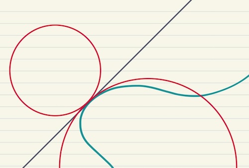
Figure: green: a curve, black: a tangent line, red: two tangent circles
These circles have the defining property that their centers lie on the line perpendicular to the tangent line. In fact, for any point on that line except for the point where the tangent and “normal” lines intersect, there is a circle tangent to the curve having that point as its center.
Anyway, suppose that our point of interest is \(p\) and that \(q\) is another point on the curve. It’s not so hard to convince yourself that there is a unique circle (or line) tangent to \(p\) and passing through \(q\). As the point \(q\) moves along the curve, the circle (that is, its center and hence its radius) varies continuously with \(q\), since our curve is continuous. We’ll define the curvature of our curve \(\gamma\) at the point \(p\) to be the limit as \(q\) approaches \(p\), of \(\frac{1}{R}\), where \(R\) is the radius of the circle through \(q\) and tangent to \(p\). In the case of a line, we’ll define the “radius” of a line to be \(\infinity\), hence its version of \(\frac{1}{R}\) should be \(0\).
It’s pretty easy to see, by computing the “mathematician examples”, that this definition satisfies our definitions.
Mathematician examples? they’re a whole thing. If you go to talks or classes given by mathematicians, they often give the silliest examples to illustrate their definition. They’re not illuminating, nor do they show the difficulty or ease of applying the definition, and yet culturally we somehow feel compelled to give them.
So: suppose \(\gamma\) is a circle of radius \(R\). Then the unique circle tangent to \(p\) on \(\gamma\) and through the point \(q\) is actually the circle \(\gamma\) itself, and we see that the curvature of a circle of radius \(R\) is \(\frac{1}{R}\) at any point, which is certainly inversely proportional to its radius.
If \(\gamma\) is a line, we have essentially by fiat defined its curvature to be \(0\) everywhere. This makes a certain amount of sense too: Although no tangent circle to \(p\) passes through any point \(q\), circles of larger and larger radius tangent to \(p\) approximate the line better and better.
Let’s compute two “real” examples: the parabola \(y = x^2\) at the point \((0,0)\) and the hyperbola \(y^2 - x^2 = 1\) at the point \((0,1)\). For both of these curves, one checks, the tangent line is horizontal at this point. Therefore any tangent circle will have center on the vertical line \(x = 0\).
For an arbitrary point \(q = (x,y)\) on the curve, we want to find the $y$-coordinate of the tangent circle to \(p\) through \(q\).
For the parabola, the point \(q = (x,y)\) satisfies \(y = x^2\), and the point \(p = (0,0)\). If \((0,s)\) is the coordinate for the center of the circle, we have that \(s\), also the distance to the origin, is equal to the distance to \(q\), which is \(\sqrt{ x^2 + (y - s)^2)} = \sqrt{y + (y - s)^2} = s\). Squaring both sides we have \(y + (y - s)^2 = s^2\), so \(y + y^2 - 2ys + s^2 = s^2\). Subtract \(s^2\) from both sides and solving for \(s\), we get \(s = (y + 1)/2\).
As the point \(q\) approaches \(p\), we have that \(y\) goes to zero, so the limiting circle has radius \(\frac{1}{2}\), and the curvature of the curve \(y = x^2\) at \((0,0)\) is therefore \(2\).
For the hyperbola, the point \(q = (x,y)\) satisfies \(y^2 - x^2 = 1\), and the point \(p\) is \((0,1)\). Again, the coordinate for the center of the circle will be \((0, s + 1)\), and we have \(s = \sqrt{x^2 + (y - s - 1)^2}\). Squaring and substituting \(x^2 = y^2 - 1\), we get \(s^2 = y^2 - 1 + (y - s - 1)^2 = y^2 - 1 + (y-1)^2 - 2(y-1)s + s^2\). Solving for \(s\), we get \(s = \frac{y^2 + (y-1)^2 - 1}{2(y - 1)}\). Notice that \(y^2 - 1 = (y - 1)(y + 1)\), so we have \(s = y\). As \(q\) approaches \(p\), we have \(y \to 1\), so the curvature of the hyperbola at \((0,1)\) is \(1\).
In fact, suppose that \(p = (x, y)\) is an arbitrary point on the hyperbola \(y^2 - x^2 = 1\). If it is on the “upper” sheet, we may assume that \(y > 0\), and therefore \(y = \sqrt{1 + x^2}\). The tangent line therefore has slope equal to the derivative of this function at \(x\), namely \(\frac{x}{1 + x^2} = \frac{x}{y}\). That is, one equation for this tangent line is \((x + ty, y + tx)\). Woah, that’s actually so neat. The line \(((1 + t)x, (1 - t)y)\) is orthogonal to this line. Fixing \(t\), the distance from this point to \((x, y)\) is \(t\sqrt{x^2 + y^2}\). Let \(q = (r,s)\) be another point on the hyperbola \(y^2 - x^2 = 1\). The distance equation, after squaring, becomes
\[\begin{align*} t^2(x^2 + y^2) &= (r - (1 + t)x)^2 + (s - (1 - t)y)^2 \\ &= r^2 + s^2 - 2rx(1+ t) - 2sy(1 - t) + x^2(1 + t)^2 + y^2(1 - t)^2 \\ \end{align*}\]
Using \(y^2 = x^2 + 1\) we can group \(t^2\) terms and get
\[\begin{align*} 2t - 2x^2 - 1 &= r^2 + s^2 - 2rx(1+t) - 2sy(1 - t) \\ \implies 2(1 + rx - sy)t &= 2x^2 + 1 + r^2 + s^2 - 2rx - 2sy \\ \implies t &= \frac{x^2 + r^2 + 1 - rx - sy}{1 + rx - sy} \end{align*}\]
Now, as \((r,s)\) approaches \((x,y)\), say \(r = x + \epsilon\) and \(s = \sqrt{1 + (x + \epsilon)^2}\), the term on the right is
\[\begin{align*}\lim_{\epsilon \to 0}\frac{x^2 + (x + \epsilon)^2 + 1 - x(x + \epsilon) - \sqrt{(1 + x^2)(1 + (x + \epsilon)^2)}}{1 + x(x + \epsilon) - \sqrt{(1 + x^2)(1 + (x + \epsilon)^2)}} \\ = \lim_{\epsilon \to 0}\frac{x^2 + x\epsilon + \epsilon^2 + 1 - \sqrt{(1 + x^2)(1 + x^2 + 2x\epsilon + \epsilon^2)}}{x^2 + x\epsilon + 1 - \sqrt{(1 + x^2)(1 + x^2 + 2x\epsilon + \epsilon^2)}} = 1. \end{align*}\]
Sorry for doing the entire calculation—briefly I was worried because if you naively set \(r = x\) and \(s = y\), the equation \(y^2 - x^2 = 1\) tells you that the numerator and denominator of the fraction computing \(t\) are both zero.
Anyway, that’s pretty neat! The hyperbola \(y^2 - x^2 = 1\) and the circle \(x^2 + y^2 = 1\) are both curves with curvature everywhere equal to \(1\).
1.4. Signed curvature?
We should be able to tell the hyperbola and the circle apart from each other based on their curvature. To do this, let’s introduce a sign to our notion of curvature. Regardless of how we parametrize our curve, there’s an orientation of it—a notion of forward. That means the tangent line has an orientation too, as does the normal line orthogonal to it: for the latter, let’s say we swing counterclockwise ninety degrees. So for the parabola at \(p = (0,0)\), and the hyperbola and circle at \(p = (0, 1)\), when the orientation of the curve has forwards pointing to the right (i.e. horizontal with increasing \(x\)), the normal will be vertical with increasing \(y\). Let’s (arbitrarily) say that the curvature is positive if the line segment from the center of the osculating (i.e. limiting) circle to the point \(p\) is positively oriented and that the curvature is negative otherwise.
This is a choice! But it has the pleasing side effect that the curvature of a circle is positive, while the curvature of the parabola and hyperbola are negative.
By the way, I found some lecture notes that give a proof of the following neat fact.
Theorem. Let \(\kappa\colon (a,b) \to \mathbb{R}\) be an integrable function. There exists a curve \(\alpha \colon (a,b) \to \mathbb{R}^2\) whose (signed) curvature function is \(\kappa\), and moreover if \(\alpha’\) is another such curve, then there exists a rigid motion of \(\mathbb{R}^2\) taking \(\alpha\) to \(\alpha’\).
In English, this says that (half of) the hyperbola \(y^2 - x^2 = 1\) is essentially the unique curve in \(\mathbb{R}^2\) whose signed curvature function is \(-1\)! I think that’s super cool.